Data Search Assignment

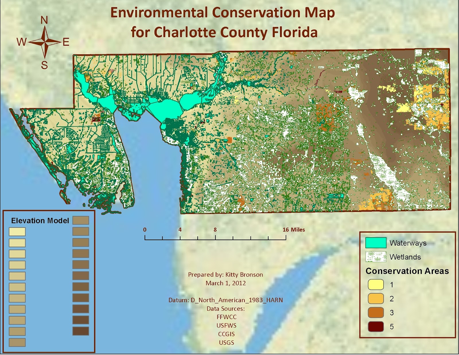
 I had a really hard time this week again, partly due to starting so late finishing up last week's assignment.  I had a frustrating first few tries and finally just dumped all my data and started fresh.  I found that if I took a look at all the medadata first and made sense of the Projections first then it is much easier.  I was assigned Charlotte County which is a western mid-state coastal county. I split the required information into two maps. One for Community Areas and one for Environmental. 

I really enjoyed working on the Environmental map and would have loved more time to do more with it.  Once I started fresh and tried my new strategy it all came together really easily.

The Community Areas map was more frustrating and I am not very happy with it.  Most of the layers came together pretty easily except the town layer I downloaded just did not work the way I thought it would, I didn't like it, it did not add to the information well so I deleted it.  The roads layer did not work at all for me.  I downloaded two separate layers, one of the layers we have worked with before and one that was the same projection/datum as some of my other layers like 'waterways' and from the same source and it still didn't work. By then I was out of time.  I did find it interesting that all the community amenities, points of interest and parks were in one section of the county (the coast which makes sense) but there is almost nothing in the eastern part of the county.

As I did last week, I will be working on the map again during this weekend and figure out my problem before I jump into next week's assignment.  I figure if I don't "get" where I am going wrong and keep moving through the assignments I will get to a place where I am truly behind and completely lost...so here goes some extra hours to fit in this weekend.

1)     County boundary

o   Source: FGDL

o   Year:2011

§  File path: S:\DataSearch\Environmental\cntbnd_jun11

·       Projection:  Albers

·       Datum: D_North_American_1983_HARN

·       Units:  Meters

2)     Cities & Towns

o   Source: CCGIS

o   Year:

§  File path: S:\DataSearch\Community\Townships

·       Projection:

·       Datum: State Plane Florida West NAD83

·       Units:  Meters

3)     Public land (Parks)

o   Source: CCGIS

o   Year:

§  File path: S:\DataSearch\Community\Parks

·       Projection:

·       Datum: State Plane Florida West NAD83

·       Units:  Meters

4)     Public land (Points of Interest)

o   Source:  CCGIS

o   Year:

§  File path: S:\DataSearch\PointsofInterest

·       Projection:

·       Datum: State Plane Florida West NAD83

·       Units:  Meters

5)     Public land (Community Amenities)

o   Source: CCGIS

o   Year:

§  File path: S:\DataSearch\Community\Community_Amenities

·       Projection:

·       Datum: State Plane Florida West NAD83

·       Units:  Meters

6)     Roads

o   Source: CCGIS

o   Year:

§  File path: S:\DataSearch\Streets

·       Projection:   

·       Datum: State Plane Florida West NAD 83

·       Units:  Meters

7)     Surface water (hydrography) Waterways

o   Source: CCGIS

o   Year:

§  File path: S:\DataSearch\Waterways

·       Projection:

·       Datum: State Plane Florida West NAD 83

·       Units:  Meters

8)     [Environmental layer 1] Strategic Habitat Conservation Areas Priority Rankings

o   Source: FFWCC (FGDL.org)

o   Year: 2009

§  File path: S:\DataSearch\SHCA_PRIO_09

·       Projection: Albers Conical Equal Area

·       Datum: D_North_American_1983_HARN

·       Units:  Meters

9)     [Environmental layer 2] National Wetlands Inventory for Florida

o   Source: USFWS (FGDL.org)

o   Year: 2011

§  File path: S:\DataSearch\NWIP_FEB11

·       Projection: Albers Conical Equal Area

·       Datum: D_North_American_1983_HARN

·       Units:  Meters

10)  [Environmental layer 2] Soils

o   Source: CCGIS

o   Year: 1984

§  File path: S:\DataSearch\Environment\Soils

·       Projection:

·       Datum: State Plane Florida West NAD83

·       Units:  Meters

11)  DOQQ

o   Source: Labins.org

o   Year:

§  File path: S:\DataSearch\Community\Aerials\q2415ne.sid (nw,se,sw)

§  File path: S:\DataSearch\Community\Aerials\q2415ne.sdw (nw,se,sw)

·       Projection: Albers

·       Datum: HPGN (NAD83)

·       Units:  Meters

·       2415 Bermont

12)  DEM

o   Source: USGS

o   Year: 1984

§  File path: S:\DataSearch\Environment\DEM

·       Projection: Albers Conical Equal Area

·       Datum: D_North_American_1983_HARN

·       Units:  Meters

PART III: Process Summary Details

1)     Added DEM file as layer

2)     Added County boundary layer

3)     Added Wetlands vector file as layer

4)     Clipped DEM raster using ‘extract by mask’ tool to match county

5)     Clipped Wetland vector using ‘clip’ tool to match county

6)     Added Strategic Habitat Conservation Areas as layer

7)     Clipped Strategic Habitat raster using ‘extract by mask’ tool to match county

8)     Added Waterways polygon from CCGIS

9)     Clipped Waterways to match county

10)  Added essential elements

11)  Saved and exported as S:\DataSearch\EnvironmentalMap_cmb.jpg

12)  Added County Boundary to new map

13)  Added Aerials for Bermont to layer

14)  Added County Parks with reprojections to match boundary

15)  Added Points of Interest layer with reprojections to match boundary

16)  Added Water layer but it was to cluttered so took away.

17)  Added Township Borders but that looked too cluttered, as well, so took away.

18)  Added two different layers of roads but neither would show up no matter what I did, one wouldn’t show up at all, the other was out in the Atlantic. 

19)  Saved file and exported as S:\DataSearch\Community.jpg

Projections Part II Lab

I had a lot of problems with this lab, hence how late it is.  I must have started over half a dozen times and spent over 20 hours on the lab.  Finally, after working late Sunday evening I erased everything after the last time it didn't work.  Monday, I reread all the previous assignments and I started totally fresh again.  The first thing I realized was that I was having problems with my layers and did a simple change in color and all the aerials and vectors lined up. I think I had gotten so confused trying to make it work that my reprojections were all wrong.  Once I had the aerials and vector layers set, I saved the .mxd and tackled the x,y coordinates.  I started from scratch with the excel file and I realized my mistake, I had the xcoord and ycoord in the wrong location.  I flipped them from what I had previously and voila...it worked! I then proceeded to finish the map and like how it came out but wish I hadn't lost so much time.

 

















Process Summary:

1)     Part 1 Practice – Downloading Data and Defining Projections

1.     Followed instructions , choosing DOQQ from Labins.org and downloading the raster and spatial reference files.

2.     Recorded the information above for files, projection, datum and units

3.     Selected the spatial reference: Projected Coordinate Systems – State Systems – NAD 1983 HARN Florida GDL Albers (Meters).prj for all 4 files.

4.     Checked the scale, units and compared to basemap

2)     Step 4 from Labins.org, selected DRG, State Plane – NAD83-Tiff-Collars Removed – Pace Quad

1.     Recorded the information above for files, projection, datum and units

2.     Selected the spatial reference – Projected Coordinate System – State Plane – NAD 1983 US Feet – NAD 1983 StatePlane Florida North FIPS 0903 USFeet.Prj

3.     Added to ArcMap and said yes to creating pyramids

4.     Checked scale, units and compared to basemap

3)     Step 5 from FTP.PGDL.org, downloaded cntbnd_jun11.zip

1.     In ArcCatalog, for cntbnd_jun11.shp, recorded name, projection, linear unit, geographic coordinate system and datum above.

4)     Part 2 Practice – Creating XY tabular data

1.     Created excel file table as instructed from original latitude and longitude data

2.     Used formula to come up with decimal degrees

3.     Saved file as S:\Projections_PartII.xls

4.     Added XY Data to ArcMap, selected Sheet1$ and added.

5.     Specified the ‘xfield’ and’ yfield’ as ‘xcoord’ and ‘ycoord’

6.     Edited coordinate system to ‘Geographic Coordinate System’ – ‘World’ – ‘WGS1984.prj’

7.     Created a shapefileby selected ‘export data’ and named S:\ProjectionsPartII\EagleNest.shp

5)     Part 3: Projection Assignment

1.     Downloaded aerials from DOQQs

2.     Selected 2004 RGB StatePlane – Untis:FT MrSID

3.     Created layers and reprojected all to output coordinate system = NAD_1983 StatePlane Florida_North_FIPS_0903_Feet

1.     aerials

2.     Major roads

3.     County boundaries

4.     Quad index

4.     Added ExcambiaSTCM.xls from R:drive

5.     Calculated the decimal degrees  Latitude = (L2+(M2/60)+(N2/3600)) and Longitude =-(O2+(P2/60)+(Q2/3600))

6.     Reprojected using ‘NAD_1983_to_WGS_1984_5’

7.     I redid the previous steps over and over again. I realized that I was making 3 major mistakes. The first mistake I figured out was that I had misunderstood the directions and had the reference system for reprojecting for the previous practice assignments.  Then I finally realized that the xy data was wrong when I specified the fields, I had the XCOORD and YCOORD backwards.  Finally, I realized that the problem with the quad layer had to do with the selection of the symbol so that it covered over the rest of the map images.  It took me several hours over a couple days more work to realize these were the mistakes.  I found that I understood the concepts but was misunderstanding the specifics of the data.

8.     Once I got the layers correct, I added the usual essential information and saved it as ProjectionsAssignmentqrctanks.mxd and exported it as ProjectionsAssignmentqrctanks.jpg to my S:drive and H:drive.

Projections Part 1 Lab

This week's lab worked with map projections in ArcGIS, along with creating the three different projection maps of the square mile area of Florida counties, we also modified the projections in ArcCatalog.

Here is my map with the three projections and relevant information.

 

















Process Summary:

1. We started with working with ArcToolox by expanding the 'Data Management Toolbox' and the 'Projections and Transformations' toolset, selecting the 'Feature' toolset and the 'Project' tool.
2. Once we had the 'Project' tool open, we set 'cntbnd' as the 'Input Dataset', 'cntbnd_utm16' as the 'Output Dataset' and then moving on to creating the new dataset by opening the 'Output Coordinate System' and then selecting 'NAD 183 UTM Zone 16N' under the Projected Coordinate System .
3. Back in the 'Project' tool window, we selected 'NAD_1983_To_Harn_Florida'
4. 'cntbnd_utm16' was added as a layer although the Geographic Coordinate System Warning did not appear even though I backed up the steps and tried it again.
5. Inserted new data frames and named these layers "Albers", "UTM" and "State Plane N." and moved the 'cntbnd_utm16' layer into the 'UTM' frame, removing it from 'Albers'.
6. Created a new layer and named it "cntbnd_stateplanen" using the Florida State Plane North projection.
7. For all the layers, a new field called "area" was created, using the 'calculate geometry' box to add the data to the new field.  I was having a bit of problems with this process, as were a couple of my classmates, but I finally got it to work.
8. Once that was accomplished it was time to put the map together, selecting the Alachua, Escambia, Polk and Miami-Date counties and add their information to the map along with the other essential data.
9. The combined layers with information on the map were saved and exported as "projections_cmb1.jpg" to my H:drive and S:drive.
10. Proceeded on to the Raster projection step.

Queensland Flooding Event

I found this article very interesting, more about policy and how the impact of devegetation made the situation worse how development on the flood plain is a big issue.

http://www.wildlife.org.au/news/2011/flooding5.html

Environmental Impact of Floods - February 2011

Dirty water reaches northern part of Moreton island. Photo ©Healthy Waterways While the massive-clean up is well underway in Queensland, the full environmental impact of the floods is still being assessed. The recent floods have devastated much of the Queensland landscape. Only time will tell how our ecosystems will bounce back from this natural disaster. Floods are a natural part of the Queensland environment but the widespread and intense nature of the current floods affecting around 80% of the state is unprecedented. It is too early to tell the full extent of the impact; the reality is we may never know. We do know that while some species will thrive others may have been killed or forcibly relocated to higher ground. Scientists suggest that ground dwelling fauna such as small mammals and reptiles may be the worst hit. The health of our waterways has been impacted significantly as many rivers and creeks were eroded, contaminated and littered with debris. Large numbers of fish have died left stranded as waters receded. The erosion of river banks is of particular concern for freshwater turtles such as the Mary River and Fitzroy River turtles. Exotic species such as carp, tilapia and red slider turtles may have spread with the floodwaters. Many riparian zones were damaged from rapid flowing water which striped away vegetation and exposed soils making them more prone to rapid erosion from future rains. The foolishness of clearing riverine vegetation has now been exposed.   Soils and waterways may have been contaminated by chemicals from nearby industrial and commercial premises – this is of particular for food producers. During the floods only 15% of the states 57 coal mines were fully operational. The coal industry lobbied the Government to temporarily drop environmental regulations and allow 44 mines to pump out millions of litres of contaminated floodwater into creeks and rivers. A large number of permits were issued. One can only contemplate the impact of such a huge release of highly toxic materials on our waterways. The current approval process and assessment criteria have clearly failed to stop environmental harm from occurring. The Government must review the current regulations. The floods should be a wake-up call to the Government about its attitude to development approvals. The Government has been warned repeatedly about approving development in flood plains but still it is allowed to happen. It is the public and ordinary folk in the high-risk areas who carry the burden of these poor planning decisions. No doubt Governments will continue this practice, if so they must lift the standards of design and enforce enhanced regulation. The flow on effects of high volumes of fresh water, sediments, nutrients, pesticides and other contaminants in waterways poses a huge threat to marine environments such as Moreton Bay, the Great Sandy and Great Barrier Reef marine parks. Mangrove habitats are particularly susceptible as they act as a net catching sediment and all sorts of debris often causing damage to their root systems. Toxic flood plumes are expected to have a significant impact on seagrass beds, corals and wetlands. Excessive silt and sediments will smother corals and seagrasses. The widespread nature of the plume will also limit the ability of species such as dugong and sea turtles to find alternative food and could cause malnutrition and death. High sediment and nutrient loads can result in algal blooms and increased disease and mortality of many marine species. Excessive scouring of riverbeds could expose acid sulphate soils which wash into the marine environment. The toxic flood plume covering much of the coast poses a threat to the Queensland seafood industry with species like prawns expected to be heavily impacted. In Moreton Bay, voluntary halts on fishing continued for weeks after the flooding event. The Government is currently evaluating and assessing the environmental impacts of the floods. It is inevitable that the environment will suffer significant short and long term impacts. There will be numerous flow-on effects as we start to see many environmental programs cut back as dollars are directed to rebuilding the state. The Gillard Government has already proposed cuts to climate change programs in order to fund flood recovery. The flood recovery must be a green recovery and cutting greenhouse gas reduction programs to fund it is not a smart solution. While no single extreme weather event can be directly attributed to climate change, the recent floods are consistent with what climate scientists have been warning for decades. If we cut carbon pollution we can reduce the severity of extreme weather events and help protect our people and our economy. Calling for the building of new dams is not the solution. We must look at ways to redevelop our cities smarter, greener and more resilient to the impacts of extreme weather events such as this. Reassessing design and development regulations must be part of the solution. Traditional catchment management has concentrated on preventing floods. We need to look at alternatives by focusing on minimising the damage rather than the occurrence. There is a need to identify ways of living and working in flood prone areas, while protecting high value assets. People living in flood prone areas should be helped to be ‘flood ready’, similar to people living in bushfire risk areas. If we can learn to accept that floods are a part of the natural cycle in the Australian climate, we can become better equipped to deal with them when they occur. I found this mapping information to be pretty good, very simple and easy to find the rainfall amounts per day.